北京大学R语言教程(李东风)第43章：基于树的方法

43.1 树回归的简单演示

决策树方法按不同自变量的不同值，分层地把训练集分组。每层使用一个变量，所以这样的分组构成一个二叉树表示。为了预测一个观测的类归属，找到它所属的组，用组的类归属或大多数观测的类归属进行预测。这样的方法称为决策树(decision tree)。决策树方法既可以用于判别问题，也可以用于回归问题，称为回归树。

决策树的好处是容易解释，在自变量为分类变量时没有额外困难。但预测准确率可能比其它有监督学习方法差。

改进方法包括装袋法(bagging)、随机森林(random forests)、提升法(boosting)。这些改进方法都是把许多棵树合并在一起，通常能改善准确率但是可解释性变差。

对Hitters数据，用Years和Hits作因变量预测log(Salaray)。

library(tidyverse)
library(ISLR) # 参考书对应的包

data(Hitters)
da_hit <- na.omit(Hitters); dim(da_hit)

## [1] 263  20

library(rsample)
set.seed(101)
hit_split <- initial_split(
  da_hit, prop = 0.80, strata = Salary)
hit_train <- training(hit_split)
hit_test <- testing(hit_split)

在训练集上建立完整的树:

library(tree)
tr1 <- tree(
  log(Salary) ~ Years + Hits, 
  data = hit_train)

剪枝为只有3个叶结点:

tr1b <- prune.tree(tr1, best=3)

显示树:

print(tr1b)

## node), split, n, deviance, yval
##       * denotes terminal node
## 
## 1) root 208 161.20 5.936  
##   2) Years < 4.5 72  35.07 5.162 *
##   3) Years > 4.5 136  60.05 6.346  
##     6) Hits < 117.5 70  23.60 5.986 *
##     7) Hits > 117.5 66  17.75 6.728 *

显示概括:

print(summary(tr1b))

## 
## Regression tree:
## snip.tree(tree = tr1, nodes = c(6L, 2L))
## Number of terminal nodes:  3 
## Residual mean deviance:  0.3727 = 76.41 / 205 
## Distribution of residuals:
##    Min. 1st Qu.  Median    Mean 3rd Qu.    Max. 
## -2.2280 -0.3740 -0.0589  0.0000  0.3414  2.5010

做树图:

plot(tr1b); text(tr1b, pretty=0)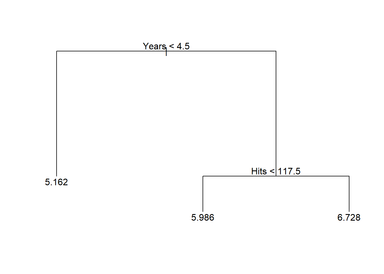

树的深度(depth)是指从根节点到最远的叶节点经过的步数，比如，上图的树的深度为2，为了用叶结点给出因变量预测值，最多需要2次判断。

43.2 树回归

树的深度是一个复杂度指标，是判别树的超参数，需要调优。关于如何进行超参数调优并在测试集上计算性能， tidymodels有系统的方法，参见47.3。这里为了对方法进行更直接的演示，直接调用交叉验证函数进行超参数调优并在测试集上计算预测精度指标。

对训练集上的未剪枝树用交叉验证方法寻找最优大小：

cv1 <- cv.tree(tr1)
print(cv1)

## $size
## [1] 9 8 6 5 4 3 2 1
## 
## $dev
## [1]  78.50049  81.47727  81.43670  79.43120  79.07190  92.16026 105.14082 167.75233
## 
## $k
## [1]      -Inf  2.445601  2.639571  3.186007  4.133744  8.296626 18.711912 66.037022
## 
## $method
## [1] "deviance"
## 
## attr(,"class")
## [1] "prune"         "tree.sequence"

plot(cv1$size, cv1$dev, type='b')
best.size <- cv1$size[which.min(cv1$dev)[1]]
abline(v=best.size, col='gray')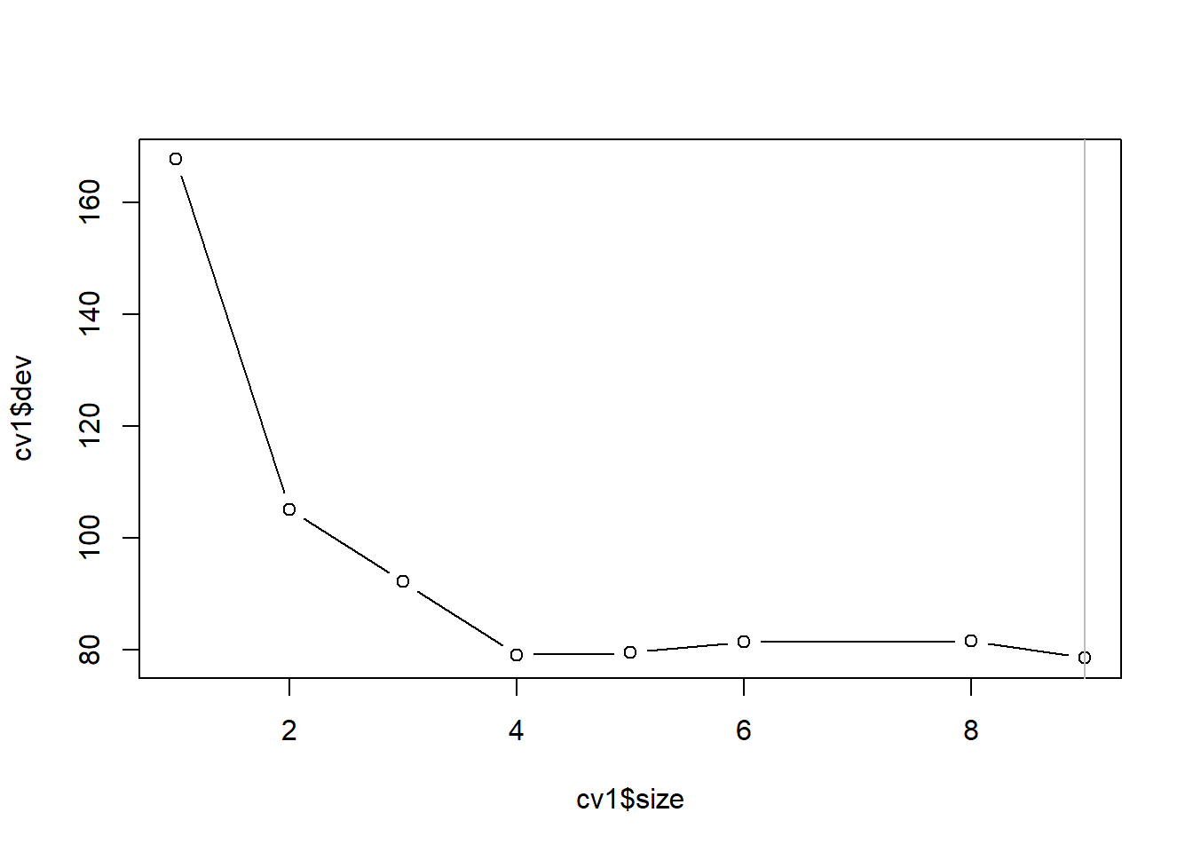

最优大小为9。但是从图上看，大小4的树已经效果很好。

获得训练集上构造的树剪枝后的结果：

tr1b <- prune.tree(tr1, best=best.size)

在测试集上计算预测根均方误差:

pred.test <- predict(tr1b, newdata = hit_test)
test.rmse <- 
  mean( (hit_test$Salary - exp(pred.test))^2 ) |> sqrt()
test.rmse

## [1] 281.7956

RMSE=281.8，比子集回归、岭回归(RMSE=240.7)、lasso的结果都差很多。

用训练集的因变量平均值估计测试集的因变量值可以作为一个最初等的用来对比的基准，其根均方误差为:

worst.rmse <- 
  mean( (hit_test$Salary - mean(hit_train$Salary))^2 ) |>
  sqrt()
worst.rmse

## [1] 413.1353

用所有数据来构造未剪枝树：

tr2 <- tree(log(Salary) ~ ., data = hit_train)

用训练集上得到的子树大小剪枝：

tr2b <- prune.tree(tr2, best=best.size)
plot(tr2b); text(tr2b, pretty=0)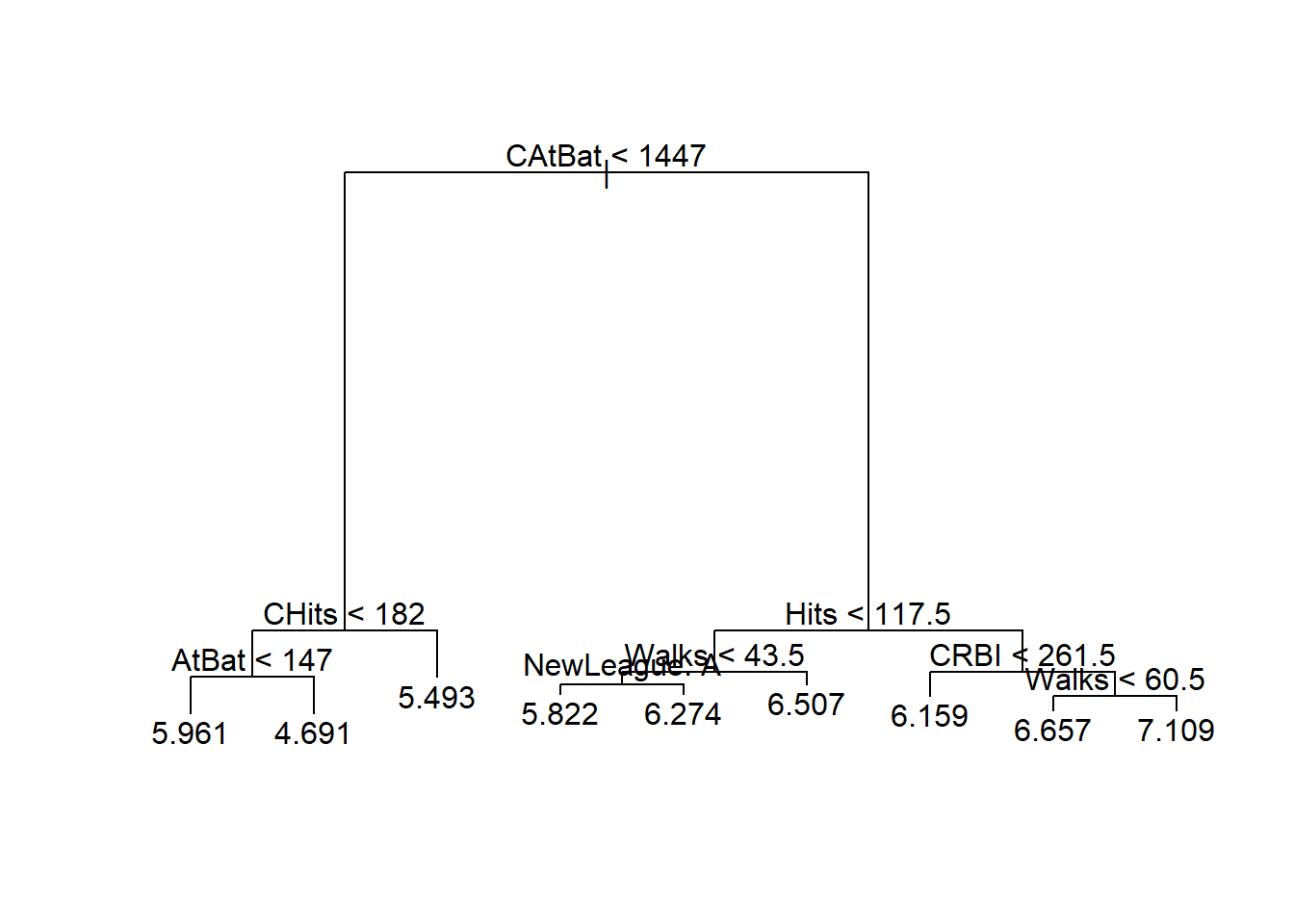

这样的结果可以用于同一问题的新数据的预测。

43.3 装袋法

判别树在不同的训练集、测试集划分上可以产生很大变化，说明其预测值方差较大。利用bootstrap的思想，可以随机选取许多个训练集，把许多个训练集的模型结果平均，就可以降低预测值的方差。

办法是从一个训练集中用有放回抽样的方法抽取B个训练集，设第b个抽取的训练集得到的回归函数为f̂ ∗b(⋅), 则最后的回归函数是这些回归函数的平均值:

f̂ bagging(x)=1B∑b=1bf̂ ∗b(x).

这称为装袋法(bagging)。装袋法对改善判别与回归树的预测精度十分有效。

装袋法的步骤如下：

从训练集中取B个有放回随机抽样的bootstrap训练集，B取为几百到几千之间。
对每个bootstrap训练集，估计未剪枝的树。
如果因变量是连续变量，对测试样品，用所有的树的预测值的平均值作预测。
如果因变量是分类变量，对测试样品，可以用所有树预测类的多数投票决定预测值。

装袋法也可以用来改进其他的回归和判别方法。

装袋后不能再用图形表示，模型可解释性较差。但是，可以度量自变量在预测中的重要程度。在回归问题中，可以计算每个自变量在所有B个树中平均减少的残差平方和的量，以此度量其重要度。在判别问题中，可以计算每个自变量在所有B个树种平均减少的基尼系数的量，以此度量其重要度。

除了可以用测试集、交叉验证方法，还可以使用袋外观测的预测误差来度量模型预测精度。用bootstrap再抽样获得多个训练集时每个bootstrap训练集总会遗漏一些观测，平均每个bootstrap训练集会遗漏三分之一的观测。对每个观测，大约有B/3棵树没有用到此观测，可以用这些树的预测值平均来预测此观测，得到一个误差估计，这样得到的均方误差估计或错判率称为袋外观测估计（OOB估计）。好处是不用很多额外的工作。

对训练集用装袋法：

library(randomForest)
bag1 <- randomForest(
  log(Salary) ~ ., 
  data = hit_train, 
  mtry=ncol(hit_train)-1, 
  importance=TRUE)
bag1

## 
## Call:
##  randomForest(formula = log(Salary) ~ ., data = hit_train, mtry = ncol(hit_train) -      1, importance = TRUE) 
##                Type of random forest: regression
##                      Number of trees: 500
## No. of variables tried at each split: 19
## 
##           Mean of squared residuals: 0.1980098
##                     % Var explained: 74.44

注意randomForest()函数实际是随机森林法，但是当mtry的值取为所有自变量个数时就是装袋法。

对测试集进行预报:

pred2 <- predict(bag1, newdata = hit_test)
test.rmse2 <- 
  mean( (hit_test$Salary - exp(pred2))^2 ) |> sqrt()
test.rmse2

## [1] 202.0765

RMSE=202.1, 比判别树的281.8改进很大，比岭回归的240.7也有很大优势。

在全集上使用装袋法：

bag2 <- randomForest(
  log(Salary) ~ ., 
  data = da_hit, 
  mtry=ncol(da_hit)-1, 
  importance=TRUE)
bag2

## 
## Call:
##  randomForest(formula = log(Salary) ~ ., data = da_hit, mtry = ncol(da_hit) -      1, importance = TRUE) 
##                Type of random forest: regression
##                      Number of trees: 500
## No. of variables tried at each split: 19
## 
##           Mean of squared residuals: 0.1937377
##                     % Var explained: 75.4

变量的重要度数值和图形：各变量的重要度数值及其图形：

importance(bag2)

##              %IncMSE IncNodePurity
## AtBat     10.7883286     8.1667778
## Hits       8.4949590     8.1050931
## HmRun      3.0595593     1.9280305
## Runs       7.6675720     3.8182568
## RBI        4.5596220     5.2948207
## Walks      8.0850741     6.9407788
## Years     10.0302334     2.2203968
## CAtBat    26.2359706    77.4088339
## CHits     12.8371027    24.0757798
## CHmRun     4.4959747     4.3641893
## CRuns     14.9272144    36.1514017
## CRBI      15.6525107    11.3891366
## CWalks     6.7160244     6.5333487
## League    -0.7821402     0.2073524
## Division  -1.0121206     0.2339053
## PutOuts    0.2771301     3.7336895
## Assists   -2.5795517     1.7112880
## Errors     0.9658563     1.7447031
## NewLeague  1.2244401     0.3597582

varImpPlot(bag2)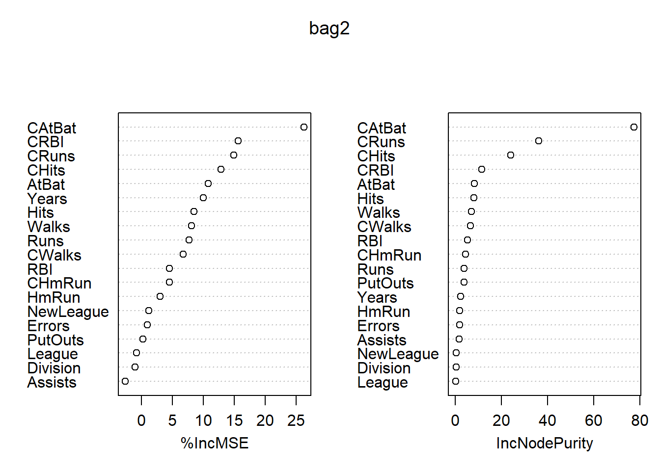

图43.1: Hitters数据装袋法的变量重要性结果

最重要的自变量是CAtBats, 其次有CRuns, CHits等。

如何计算变量重要度？基于树的方法，每个叶节点的纯度越高（叶结点中所有观测的标签相同，或者因变量值相等），模型拟合优度越好。所以，对每一个变量，可以计算其在作为分枝用的变量时，对中间节点的纯度指标的改善量，将这些改善量加起来。对装袋法、随机森林、提升法（如GBM），则是计算每个变量对损失函数的改善量。

不同的机器学习算法对变量重要程度有不同的定义，比如，广义线性模型(GLM)用标准化后的自变量的系数估计的绝对值大小作为重要程度度量。

43.4 随机森林

随机森林的思想与装袋法类似，但是试图使得参加平均的各个树之间变得比较独立，以减少正相关的预测在计算平均时的标准误差膨胀问题。仍采用有放回抽样得到的多个bootstrap训练集，但是对每个bootstrap训练集构造判别树时，每次分叉时不考虑所有自变量，而是仅考虑随机选取的一个自变量子集。这个自变量子集的自变量个数是一个模型超参数。

对判别树，每次分叉时选取的自变量个数通常取m≈p‾√个。比如，对Heart数据的13个自变量，每次分叉时仅随机选取4个纳入考察范围。

随机森林的想法是基于正相关的样本在平均时并不能很好地降低方差，独立样本能比较好地降低方差。如果存在一个最重要的变量，如果不加限制这个最重要的变量总会是第一个分叉，使得B棵树相似程度很高。随机森林解决这个问题的办法是限制分叉时可选的变量子集。

随机森林也可以用来改进其他的回归和判别方法。

装袋法和随机森林都可以用R扩展包randomForest的 randomForest()函数实现。当此函数的mtry参数取为自变量个数时，执行的就是装袋法； mtry取缺省值时，执行随机森林算法。执行随机森林算法时， randomForest()函数在回归问题时分叉时考虑的自变量个数取m≈p/3，在判别问题时取m≈p‾√。

对训练集用随机森林法：

library(randomForest)
rf1 <- randomForest(
  log(Salary) ~ ., 
  data = hit_train, 
  importance=TRUE)
rf1

## 
## Call:
##  randomForest(formula = log(Salary) ~ ., data = hit_train, importance = TRUE) 
##                Type of random forest: regression
##                      Number of trees: 500
## No. of variables tried at each split: 6
## 
##           Mean of squared residuals: 0.1895383
##                     % Var explained: 75.54

当mtry的值取为缺省值时执行随机森林算法。

对测试集进行预报:

pred3 <- predict(rf1, newdata = hit_test)
test.rmse3 <- 
  mean( (hit_test$Salary - exp(pred3))^2 ) |> sqrt()
test.rmse3

## [1] 199.8305

RMSE=199.8, 与装袋法(RMSE=202.1)相近。

在全集上使用随机森林：

rf2 <- randomForest(
  log(Salary) ~ ., 
  data = da_hit, 
  importance=TRUE)
rf2

## 
## Call:
##  randomForest(formula = log(Salary) ~ ., data = da_hit, importance = TRUE) 
##                Type of random forest: regression
##                      Number of trees: 500
## No. of variables tried at each split: 6
## 
##           Mean of squared residuals: 0.1799338
##                     % Var explained: 77.16

各变量的重要度数值及其图形：

importance(rf2)

##              %IncMSE IncNodePurity
## AtBat     10.8759999     7.4439449
## Hits       8.1725427     7.9481573
## HmRun      4.4016043     2.5935154
## Runs       9.2818801     4.8293772
## RBI        8.3514919     6.2292463
## Walks      8.8164532     6.1787450
## Years     10.6053647     5.0062719
## CAtBat    16.9507148    41.0814114
## CHits     17.6578387    41.5968368
## CHmRun     8.1292431     7.1035557
## CRuns     13.8588073    30.0948238
## CRBI      14.2775671    19.7903282
## CWalks    10.3261013    15.7222964
## League     2.0932305     0.2700378
## Division  -0.2466121     0.3021408
## PutOuts    3.1669627     3.2670212
## Assists   -0.6733127     1.7261075
## Errors     1.5649441     1.6376596
## NewLeague  1.0967640     0.3386188

varImpPlot(rf2)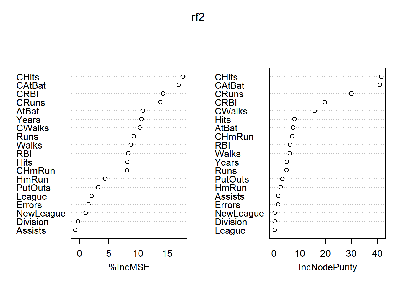

图43.2: Hitters数据随机森林法的变量重要度结果

最重要的自变量是CAtBats, CRuns, CHits, CWalks, CRBI等。

43.5 提升法

提升法(Boosting)，也称为梯度提升法，也是可以用在多种回归和判别问题中的方法。提升法的想法是，用比较简单的模型拟合因变量，计算残差，然后以残差为新的因变量建模，仍使用简单的模型，把两次的回归函数作加权和，得到新的残差后，再以新残差作为因变量建模，如此重复地更新回归函数，得到由多个回归函数加权和组成的最终的回归函数。

加权一般取为比较小的值，其目的是降低逼近速度。统计学习问题中降低逼近速度一般结果更好。

提升法算法:

[(1)] 对训练集，设置ri=yi，并令初始回归函数为f̂ (⋅)=0。
[(2)] 对b=1,2,…,B重复执行：
- [(a)] 以训练集的自变量为自变量，以r为因变量，拟合一个仅有d个分叉的简单树回归函数，设为f̂ b；
- [(b)] 更新回归函数，添加一个压缩过的树回归函数:f̂ (x)←f̂ (x)+λf̂ b(x);
- [(c)] 更新残差:ri←ri−λf̂ b(xi).
[(3)] 提升法的回归函数为f̂ (x)=∑b=1Bλf̂ b(x).

用多少个回归函数做加权和，即B的选取问题。取得B太大也会有过度拟合，但是只要B不太大这个问题不严重。可以用交叉验证选择B的值。

收缩系数λ。是一个小的正数，控制学习速度，经常用0.01, 0.001这样的值，与要解决的问题有关。取λ很小，就需要取B很大。

用来控制每个回归函数复杂度的参数，对树回归而言就是树的大小，用树的深度d表示。深度等于1则仅使用一个自变量，仅有一次分叉，就是二叉树，这样多棵树相加，相当于各个变量的可加模型，没有交互作用效应，这样的可加模型往往就很好。 d>1时就加入了交互项，比如d=2，就可以用两个变量，用叶结点预测因变量时，最多可以用两个自变量作两次判断，因为树模型是非线性的，将许多棵这样的深度为2的树相加，就可以包含自变量两两之间的非线性的相互作用效应。

gbm实现了提升法。 interaction.depth表示树的深度（复杂度）， n.trees表示用多少棵树相加。 shrinkage表示学习速度，即算法中的λ。 n.minobsinnode表示每个叶结点至少应包含的观测点数，可以设置这个参数，以避免过少的训练样例也单独作为一个规则。这些都是超参数，应进行超参数调优，这里仅固定了这些超参数进行演示。

在训练集上拟合：

library(gbm)
set.seed(1)
bst1 <- gbm(
  log(Salary) ~ ., 
  data = hit_train, 
  distribution = "gaussian",  
  n.trees=5000,  
  interaction.depth=4)
summary(bst1)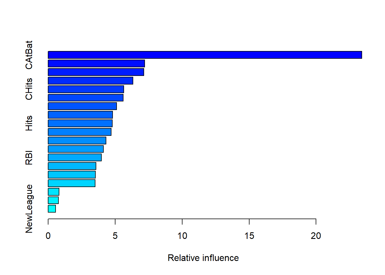

##                 var    rel.inf
## CAtBat       CAtBat 23.4075576
## CRBI           CRBI  7.2138130
## CRuns         CRuns  7.1524081
## PutOuts     PutOuts  6.3402558
## CHits         CHits  5.6558782
## CHmRun       CHmRun  5.6051624
## Walks         Walks  5.1110904
## Assists     Assists  4.8197073
## Hits           Hits  4.7970012
## CWalks       CWalks  4.7150910
## AtBat         AtBat  4.3214885
## HmRun         HmRun  4.1297511
## RBI             RBI  3.9799787
## Years         Years  3.5699618
## Runs           Runs  3.5257357
## Errors       Errors  3.5019377
## Division   Division  0.8191874
## League       League  0.7703509
## NewLeague NewLeague  0.5636432

CAtBat是最重要的变量。

在测试集上预报，并计算根均方误差：

yhat <- predict(
  bst1, 
  newdata = hit_test)

## Using 5000 trees...

mean( (hit_test$Salary - exp(yhat))^2 ) |> sqrt()

## [1] 274.633

RMSE=274.6，结果比较差，需要进行参数调优。

43.6 心脏病诊断建模预报

Heart数据是心脏病诊断的数据，因变量AHD为是否有心脏病，试图用各个自变量预测（判别）。

读入Heart数据集，并去掉有缺失值的观测：

Heart <- read_csv(
  "data/Heart.csv",
  show_col_types = FALSE) |>
  dplyr::select(-1) |>
  mutate(
    AHD = factor(AHD, levels=c("Yes", "No"))
  )

## New names:
## • `` -> `...1`

Heart <- na.omit(Heart)
glimpse(Heart)

## Rows: 297
## Columns: 14
## $ Age       <dbl> 63, 67, 67, 37, 41, 56, 62, 57, 63, 53, 57, 56, 56, 44, 52, 57, 48, 54, 48, 49, 64, 58, 58, 58, 60, 50, 58, 66, 43, 40, 69, 60, 64, 59, 44, 42, 43, 57, 55, 61, 65, 40, 71, 59, 61, 58, 51, 50, 65, 53, 41, 65, 44, 44, 60, 54, 50, 41, 54, 51, 51, 46, 58, 54, 54, 60, 60, 54, 59, 46, 65, 67, 62, 65, 44, 65, 60, 51, 48, 58, 45, 53, 39, 68, 52, 44, 47, 53, 51, 66, 62, 62, 44, 63, 52, 59, 60, 52, 48, 45, 34, 57, 71, 49, 54, 59, 57, 61, 39, 61, 56, 52, 43, 62, 41, 58, 35, 63, 65, 48, …
## $ Sex       <dbl> 1, 1, 1, 1, 0, 1, 0, 0, 1, 1, 1, 0, 1, 1, 1, 1, 1, 1, 0, 1, 1, 0, 1, 1, 1, 0, 0, 0, 1, 1, 0, 1, 1, 1, 1, 1, 1, 1, 1, 1, 0, 1, 0, 1, 0, 1, 1, 1, 0, 1, 0, 1, 1, 1, 1, 1, 1, 1, 1, 1, 0, 0, 1, 0, 1, 1, 1, 1, 1, 1, 0, 1, 1, 1, 1, 0, 1, 0, 1, 1, 1, 0, 1, 1, 1, 1, 1, 0, 0, 1, 0, 1, 0, 0, 1, 1, 0, 1, 1, 1, 1, 0, 0, 1, 1, 1, 1, 1, 1, 0, 1, 1, 0, 0, 1, 1, 0, 1, 1, 1, 0, 1, 1, 1, 0, 0, 1, 1, 0, 1, 1, 1, 1, 0, 0, 1, 1, 1, 1, 1, 1, 1, 1, 1, 1, 1, 1, 1, 0, 1, 0, 0, 1, 1, 1, 1, 1, 1, 1, 1, …
## $ ChestPain <chr> "typical", "asymptomatic", "asymptomatic", "nonanginal", "nontypical", "nontypical", "asymptomatic", "asymptomatic", "asymptomatic", "asymptomatic", "asymptomatic", "nontypical", "nonanginal", "nontypical", "nonanginal", "nonanginal", "nontypical", "asymptomatic", "nonanginal", "nontypical", "typical", "typical", "nontypical", "nonanginal", "asymptomatic", "nonanginal", "nonanginal", "typical", "asymptomatic", "asymptomatic", "typical", "asymptomatic", "nonanginal", "asymptom…
## $ RestBP    <dbl> 145, 160, 120, 130, 130, 120, 140, 120, 130, 140, 140, 140, 130, 120, 172, 150, 110, 140, 130, 130, 110, 150, 120, 132, 130, 120, 120, 150, 150, 110, 140, 117, 140, 135, 130, 140, 120, 150, 132, 150, 150, 140, 160, 150, 130, 112, 110, 150, 140, 130, 105, 120, 112, 130, 130, 124, 140, 110, 125, 125, 130, 142, 128, 135, 120, 145, 140, 150, 170, 150, 155, 125, 120, 110, 110, 160, 125, 140, 130, 150, 104, 130, 140, 180, 120, 140, 138, 138, 130, 120, 160, 130, 108, 135, 128, 110, …
## $ Chol      <dbl> 233, 286, 229, 250, 204, 236, 268, 354, 254, 203, 192, 294, 256, 263, 199, 168, 229, 239, 275, 266, 211, 283, 284, 224, 206, 219, 340, 226, 247, 167, 239, 230, 335, 234, 233, 226, 177, 276, 353, 243, 225, 199, 302, 212, 330, 230, 175, 243, 417, 197, 198, 177, 290, 219, 253, 266, 233, 172, 273, 213, 305, 177, 216, 304, 188, 282, 185, 232, 326, 231, 269, 254, 267, 248, 197, 360, 258, 308, 245, 270, 208, 264, 321, 274, 325, 235, 257, 234, 256, 302, 164, 231, 141, 252, 255, 239, …
## $ Fbs       <dbl> 1, 0, 0, 0, 0, 0, 0, 0, 0, 1, 0, 0, 1, 0, 1, 0, 0, 0, 0, 0, 0, 1, 0, 0, 0, 0, 0, 0, 0, 0, 0, 1, 0, 0, 0, 0, 0, 0, 0, 1, 0, 0, 0, 1, 0, 0, 0, 0, 1, 1, 0, 0, 0, 0, 0, 0, 0, 0, 0, 0, 0, 0, 0, 1, 0, 0, 0, 0, 0, 0, 0, 1, 0, 0, 0, 0, 0, 0, 0, 0, 0, 0, 0, 1, 0, 0, 0, 0, 0, 0, 0, 0, 0, 0, 0, 0, 0, 0, 0, 0, 0, 0, 1, 0, 0, 0, 0, 0, 0, 0, 1, 0, 1, 0, 0, 1, 0, 1, 0, 1, 0, 0, 0, 1, 0, 1, 0, 0, 0, 0, 0, 0, 0, 0, 0, 0, 0, 0, 1, 0, 0, 1, 0, 0, 0, 1, 0, 0, 0, 1, 0, 0, 0, 0, 0, 0, 0, 0, 0, 1, …
## $ RestECG   <dbl> 2, 2, 2, 0, 2, 0, 2, 0, 2, 2, 0, 2, 2, 0, 0, 0, 0, 0, 0, 0, 2, 2, 2, 2, 2, 0, 0, 0, 0, 2, 0, 0, 0, 0, 0, 0, 2, 2, 0, 0, 2, 0, 0, 0, 2, 2, 0, 2, 2, 2, 0, 0, 2, 2, 0, 2, 0, 2, 2, 2, 0, 2, 2, 0, 0, 2, 2, 2, 2, 0, 0, 0, 0, 2, 2, 2, 2, 2, 2, 2, 2, 2, 2, 2, 0, 2, 2, 2, 2, 2, 2, 0, 0, 2, 0, 2, 2, 0, 2, 2, 2, 2, 2, 0, 0, 0, 2, 0, 0, 2, 2, 2, 2, 0, 0, 2, 0, 2, 2, 2, 2, 0, 0, 2, 2, 2, 0, 0, 0, 2, 0, 2, 2, 0, 2, 0, 2, 0, 2, 0, 2, 0, 0, 2, 0, 2, 0, 2, 0, 0, 2, 2, 2, 2, 2, 0, 2, 2, 0, 0, …
## $ MaxHR     <dbl> 150, 108, 129, 187, 172, 178, 160, 163, 147, 155, 148, 153, 142, 173, 162, 174, 168, 160, 139, 171, 144, 162, 160, 173, 132, 158, 172, 114, 171, 114, 151, 160, 158, 161, 179, 178, 120, 112, 132, 137, 114, 178, 162, 157, 169, 165, 123, 128, 157, 152, 168, 140, 153, 188, 144, 109, 163, 158, 152, 125, 142, 160, 131, 170, 113, 142, 155, 165, 140, 147, 148, 163, 99, 158, 177, 151, 141, 142, 180, 111, 148, 143, 182, 150, 172, 180, 156, 160, 149, 151, 145, 146, 175, 172, 161, 142, 1…
## $ ExAng     <dbl> 0, 1, 1, 0, 0, 0, 0, 1, 0, 1, 0, 0, 1, 0, 0, 0, 0, 0, 0, 0, 1, 0, 0, 0, 1, 0, 0, 0, 0, 1, 0, 1, 0, 0, 1, 0, 1, 1, 1, 1, 0, 1, 0, 0, 0, 0, 0, 0, 0, 0, 0, 0, 0, 0, 1, 1, 0, 0, 0, 1, 1, 1, 1, 0, 0, 1, 0, 0, 1, 0, 0, 0, 1, 0, 0, 0, 1, 0, 0, 1, 1, 0, 0, 1, 0, 0, 0, 0, 0, 0, 0, 0, 0, 0, 1, 1, 0, 0, 0, 0, 0, 0, 0, 0, 0, 1, 0, 1, 0, 1, 1, 0, 1, 0, 0, 0, 0, 1, 0, 1, 0, 1, 1, 0, 0, 1, 1, 0, 0, 0, 1, 0, 1, 0, 0, 1, 0, 1, 0, 1, 0, 0, 1, 1, 0, 0, 0, 0, 0, 0, 0, 0, 1, 1, 0, 1, 0, 0, 0, 0, …
## $ Oldpeak   <dbl> 2.3, 1.5, 2.6, 3.5, 1.4, 0.8, 3.6, 0.6, 1.4, 3.1, 0.4, 1.3, 0.6, 0.0, 0.5, 1.6, 1.0, 1.2, 0.2, 0.6, 1.8, 1.0, 1.8, 3.2, 2.4, 1.6, 0.0, 2.6, 1.5, 2.0, 1.8, 1.4, 0.0, 0.5, 0.4, 0.0, 2.5, 0.6, 1.2, 1.0, 1.0, 1.4, 0.4, 1.6, 0.0, 2.5, 0.6, 2.6, 0.8, 1.2, 0.0, 0.4, 0.0, 0.0, 1.4, 2.2, 0.6, 0.0, 0.5, 1.4, 1.2, 1.4, 2.2, 0.0, 1.4, 2.8, 3.0, 1.6, 3.4, 3.6, 0.8, 0.2, 1.8, 0.6, 0.0, 0.8, 2.8, 1.5, 0.2, 0.8, 3.0, 0.4, 0.0, 1.6, 0.2, 0.0, 0.0, 0.0, 0.5, 0.4, 6.2, 1.8, 0.6, 0.0, 0.0, 1.2, …
## $ Slope     <dbl> 3, 2, 2, 3, 1, 1, 3, 1, 2, 3, 2, 2, 2, 1, 1, 1, 3, 1, 1, 1, 2, 1, 2, 1, 2, 2, 1, 3, 1, 2, 1, 1, 1, 2, 1, 1, 2, 2, 2, 2, 2, 1, 1, 1, 1, 2, 1, 2, 1, 3, 1, 1, 1, 1, 1, 2, 2, 1, 3, 1, 2, 3, 2, 1, 2, 2, 2, 1, 3, 2, 1, 2, 2, 1, 1, 1, 2, 1, 2, 1, 2, 2, 1, 2, 1, 1, 1, 1, 1, 2, 3, 2, 2, 1, 1, 2, 2, 1, 1, 1, 1, 1, 1, 2, 1, 1, 2, 2, 2, 2, 2, 2, 2, 2, 2, 1, 1, 1, 2, 1, 2, 2, 3, 2, 2, 3, 2, 1, 1, 2, 1, 1, 1, 2, 2, 3, 2, 2, 2, 1, 2, 1, 2, 2, 1, 2, 1, 1, 1, 2, 2, 2, 2, 3, 2, 1, 1, 2, 1, 1, …
## $ Ca        <dbl> 0, 3, 2, 0, 0, 0, 2, 0, 1, 0, 0, 0, 1, 0, 0, 0, 0, 0, 0, 0, 0, 0, 0, 2, 2, 0, 0, 0, 0, 0, 2, 2, 0, 0, 0, 0, 0, 1, 1, 0, 3, 0, 2, 0, 0, 1, 0, 0, 1, 0, 1, 0, 1, 0, 1, 1, 1, 0, 1, 1, 0, 0, 3, 0, 1, 2, 0, 0, 0, 0, 0, 2, 2, 2, 1, 0, 1, 1, 0, 0, 0, 0, 0, 0, 0, 0, 0, 0, 0, 0, 3, 3, 0, 0, 1, 1, 2, 1, 0, 0, 0, 1, 1, 3, 0, 1, 1, 1, 0, 0, 1, 0, 0, 1, 0, 0, 0, 3, 1, 2, 3, 0, 0, 1, 0, 2, 1, 0, 0, 0, 1, 0, 0, 0, 0, 0, 1, 0, 0, 0, 0, 0, 0, 0, 0, 3, 0, 0, 1, 0, 0, 0, 1, 1, 3, 0, 2, 2, 1, 0, …
## $ Thal      <chr> "fixed", "normal", "reversable", "normal", "normal", "normal", "normal", "normal", "reversable", "reversable", "fixed", "normal", "fixed", "reversable", "reversable", "normal", "reversable", "normal", "normal", "normal", "normal", "normal", "normal", "reversable", "reversable", "normal", "normal", "normal", "normal", "reversable", "normal", "reversable", "normal", "reversable", "normal", "normal", "reversable", "fixed", "reversable", "normal", "reversable", "reversable", "nor…
## $ AHD       <fct> No, Yes, Yes, No, No, No, Yes, No, Yes, Yes, No, No, Yes, No, No, No, Yes, No, No, No, No, No, Yes, Yes, Yes, No, No, No, No, Yes, No, Yes, Yes, No, No, No, Yes, Yes, Yes, No, Yes, No, No, No, Yes, Yes, No, Yes, No, No, No, No, Yes, No, Yes, Yes, Yes, Yes, No, No, Yes, No, Yes, No, Yes, Yes, Yes, No, Yes, Yes, No, Yes, Yes, Yes, Yes, No, Yes, No, No, Yes, No, No, No, Yes, No, No, No, No, No, No, Yes, No, No, No, Yes, Yes, Yes, No, No, No, No, No, No, Yes, No, Yes, Yes, Yes, Y…

t(summary(Heart))

##                                                                                                                       
##      Age   Min.   :29.00      1st Qu.:48.00      Median :56.00      Mean   :54.54    3rd Qu.:61.00    Max.   :77.00   
##      Sex   Min.   :0.0000     1st Qu.:0.0000     Median :1.0000     Mean   :0.6768   3rd Qu.:1.0000   Max.   :1.0000  
##  ChestPain Length:297         Class :character   Mode  :character                                                     
##     RestBP Min.   : 94.0      1st Qu.:120.0      Median :130.0      Mean   :131.7    3rd Qu.:140.0    Max.   :200.0   
##      Chol  Min.   :126.0      1st Qu.:211.0      Median :243.0      Mean   :247.4    3rd Qu.:276.0    Max.   :564.0   
##      Fbs   Min.   :0.0000     1st Qu.:0.0000     Median :0.0000     Mean   :0.1448   3rd Qu.:0.0000   Max.   :1.0000  
##    RestECG Min.   :0.0000     1st Qu.:0.0000     Median :1.0000     Mean   :0.9966   3rd Qu.:2.0000   Max.   :2.0000  
##     MaxHR  Min.   : 71.0      1st Qu.:133.0      Median :153.0      Mean   :149.6    3rd Qu.:166.0    Max.   :202.0   
##     ExAng  Min.   :0.0000     1st Qu.:0.0000     Median :0.0000     Mean   :0.3266   3rd Qu.:1.0000   Max.   :1.0000  
##    Oldpeak Min.   :0.000      1st Qu.:0.000      Median :0.800      Mean   :1.056    3rd Qu.:1.600    Max.   :6.200   
##     Slope  Min.   :1.000      1st Qu.:1.000      Median :2.000      Mean   :1.603    3rd Qu.:2.000    Max.   :3.000   
##       Ca   Min.   :0.0000     1st Qu.:0.0000     Median :0.0000     Mean   :0.6768   3rd Qu.:1.0000   Max.   :3.0000  
##     Thal   Length:297         Class :character   Mode  :character                                                     
##  AHD       Yes:137            No :160

数据下载：Heart.csv

43.6.1 划分训练集与测试集

简单地把观测分为一半训练集、一半测试集：

library(rsample)
set.seed(101)
heart_split <- initial_split(
  Heart, prop = 0.50)
heart_train <- training(heart_split)
heart_test <- testing(heart_split)
test.y <- heart_test$AHD

43.6.2 判别树

在训练集上建立未剪枝的判别树:

tr1 <- tree(AHD ~ ., data = heart_train)

## Warning in tree(AHD ~ ., data = heart_train): NAs introduced by coercion

plot(tr1); text(tr1, pretty=0)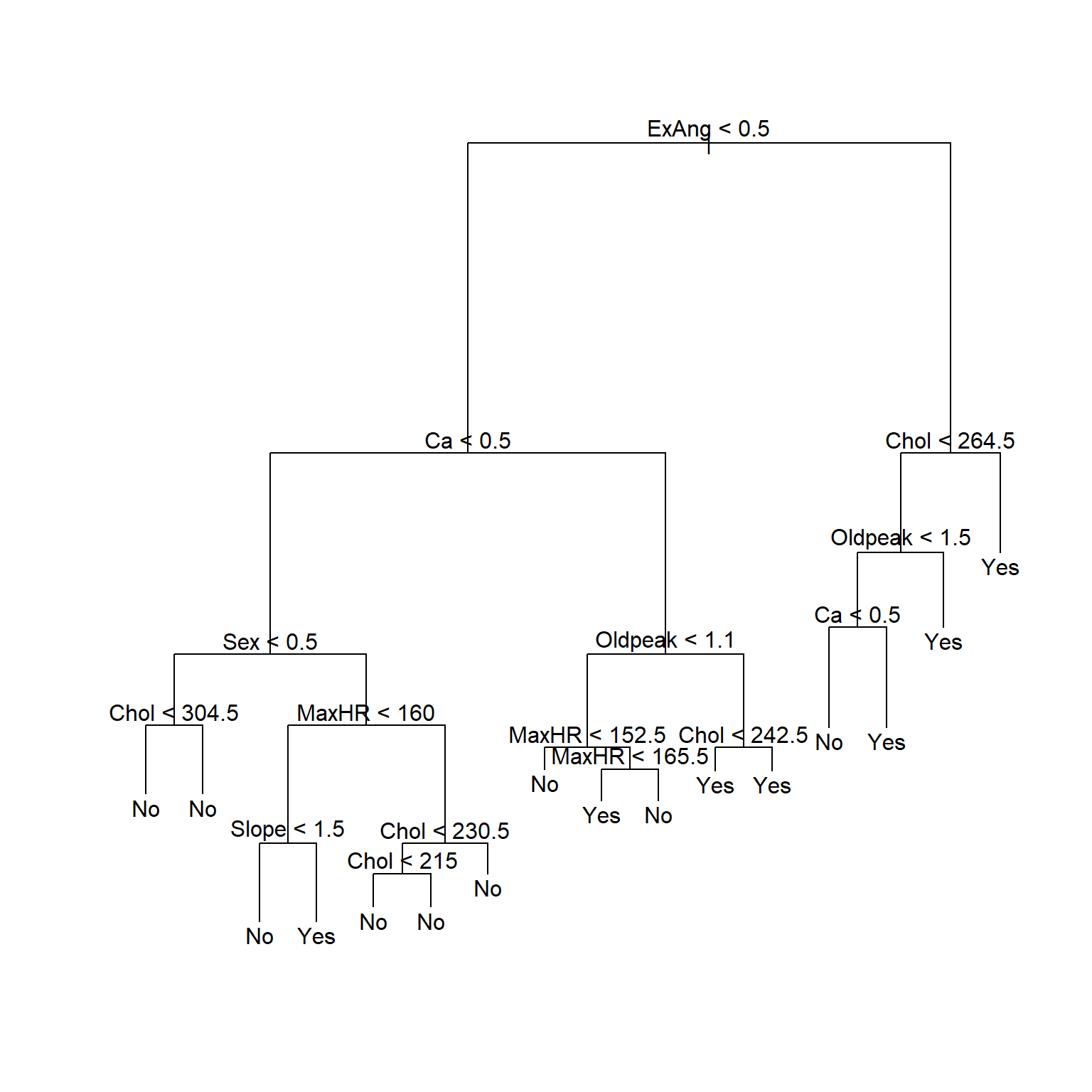

注意剪枝后树的显示中，如果内部节点的自变量存在分类变量，这时按照这个自变量分叉时，取指定的某几个分类值时对应分支Yes，取其它的分类值时对应分支No。

43.6.2.1 适当剪枝

用交叉验证方法确定剪枝保留的叶子个数，剪枝时按照错判率(等于1减去正确率)执行：

cv1 <- cv.tree(tr1, FUN=prune.misclass)

## Warning in tree(model = m[rand != i, , drop = FALSE]): NAs introduced by coercion

## Warning in pred1.tree(tree, tree.matrix(nd)): NAs introduced by coercion

## Warning in tree(model = m[rand != i, , drop = FALSE]): NAs introduced by coercion

## Warning in pred1.tree(tree, tree.matrix(nd)): NAs introduced by coercion

## Warning in tree(model = m[rand != i, , drop = FALSE]): NAs introduced by coercion

## Warning in pred1.tree(tree, tree.matrix(nd)): NAs introduced by coercion

## Warning in tree(model = m[rand != i, , drop = FALSE]): NAs introduced by coercion

## Warning in pred1.tree(tree, tree.matrix(nd)): NAs introduced by coercion

## Warning in tree(model = m[rand != i, , drop = FALSE]): NAs introduced by coercion

## Warning in pred1.tree(tree, tree.matrix(nd)): NAs introduced by coercion

## Warning in tree(model = m[rand != i, , drop = FALSE]): NAs introduced by coercion

## Warning in pred1.tree(tree, tree.matrix(nd)): NAs introduced by coercion

## Warning in tree(model = m[rand != i, , drop = FALSE]): NAs introduced by coercion

## Warning in pred1.tree(tree, tree.matrix(nd)): NAs introduced by coercion

## Warning in tree(model = m[rand != i, , drop = FALSE]): NAs introduced by coercion

## Warning in pred1.tree(tree, tree.matrix(nd)): NAs introduced by coercion

## Warning in tree(model = m[rand != i, , drop = FALSE]): NAs introduced by coercion

## Warning in pred1.tree(tree, tree.matrix(nd)): NAs introduced by coercion

## Warning in tree(model = m[rand != i, , drop = FALSE]): NAs introduced by coercion

## Warning in pred1.tree(tree, tree.matrix(nd)): NAs introduced by coercion

cv1

## $size
## [1] 16 12  6  3  2  1
## 
## $dev
## [1] 51 50 53 47 57 75
## 
## $k
## [1]      -Inf  0.000000  1.666667  2.000000 12.000000 24.000000
## 
## $method
## [1] "misclass"
## 
## attr(,"class")
## [1] "prune"         "tree.sequence"

plot(cv1$size, cv1$dev, type='b', xlab='size', ylab='dev')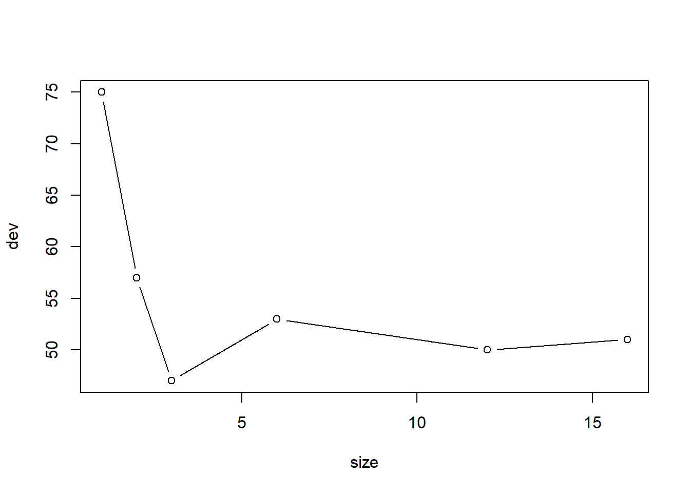

best.size <- cv1$size[which.min(cv1$dev)]

最优的大小是3。

对训练集生成剪枝结果：

tr1b <- prune.misclass(tr1, best=best.size)
plot(tr1b); text(tr1b, pretty=0)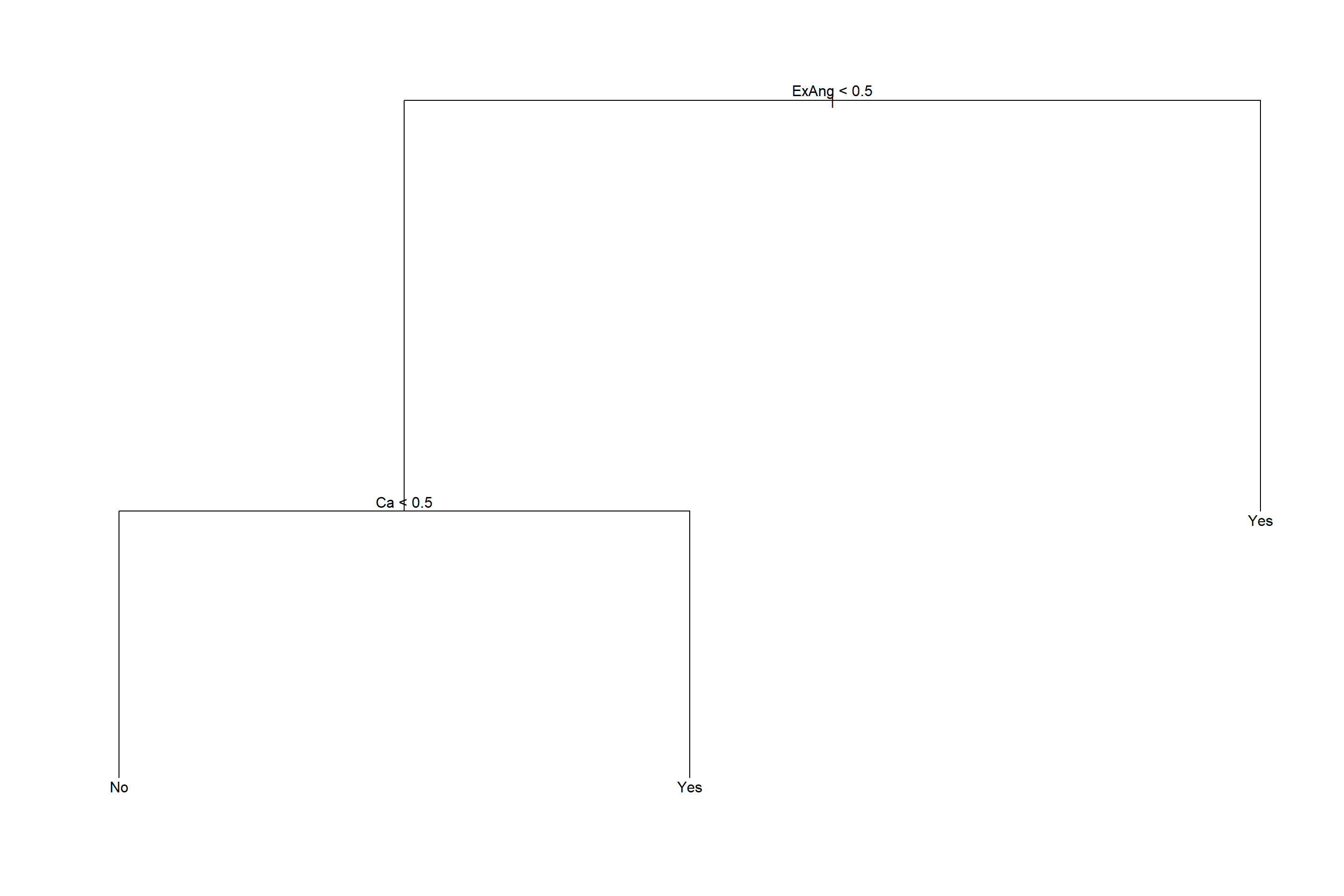

图43.3: Heart数据回归树

43.6.2.2 对测试集计算误判率

pred1 <- predict(tr1b, heart_test, type='class')

## Warning in pred1.tree(object, tree.matrix(newdata)): NAs introduced by coercion

tab1 <- table(pred1, test.y); tab1

##      test.y
## pred1 Yes No
##   Yes  52 30
##   No    6 61

test.err <- (tab1[1,2]+tab1[2,1])/sum(tab1[]); test.err

## [1] 0.2416107

对测试集的错判率约24%。

利用未剪枝的树对测试集进行预测, 一般比剪枝后的结果差:

pred1a <- predict(tr1, heart_test, type='class')

## Warning in pred1.tree(object, tree.matrix(newdata)): NAs introduced by coercion

tab1a <- table(pred1a, test.y); tab1a

##       test.y
## pred1a Yes No
##    Yes  42 25
##    No   16 66

test.err1a <- (tab1a[1,2]+tab1a[2,1])/sum(tab1a[]); test.err1a

## [1] 0.2751678

43.6.2.3 利用全集数据建立剪枝判别树

tr2 <- tree(AHD ~ ., data=Heart)

## Warning in tree(AHD ~ ., data = Heart): NAs introduced by coercion

tr2b <- prune.misclass(tr2, best=best.size)
plot(tr2b); text(tr2b, pretty=0)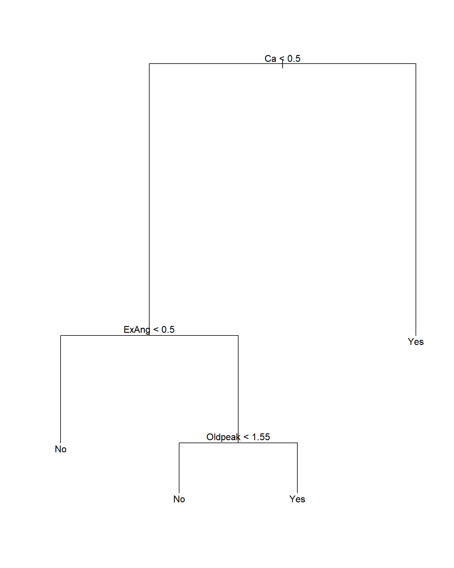

43.6.3 用装袋法

对训练集用装袋法：

bag1 <- randomForest(
  AHD ~ ., 
  data = heart_train, 
  mtry=13, 
  importance=TRUE)
bag1

## 
## Call:
##  randomForest(formula = AHD ~ ., data = heart_train, mtry = 13,      importance = TRUE) 
##                Type of random forest: classification
##                      Number of trees: 500
## No. of variables tried at each split: 13
## 
##         OOB estimate of  error rate: 23.65%
## Confusion matrix:
##     Yes No class.error
## Yes  61 18   0.2278481
## No   17 52   0.2463768

注意randomForest()函数实际是随机森林法，但是当mtry的值取为所有自变量个数时就是装袋法。袋外观测得到的错判率比较差。

对测试集进行预报:

pred2 <- predict(bag1, newdata = heart_test)
tab2 <- table(pred2, test.y); tab2

##      test.y
## pred2 Yes No
##   Yes  44 15
##   No   14 76

test.err2 <- (tab2[1,2]+tab2[2,1])/sum(tab2[]); test.err2

## [1] 0.1946309

测试集的错判率约为19%。

对全集用装袋法:

bag1b <- randomForest(
  AHD ~ ., 
  data=Heart, 
  mtry=13, 
  importance=TRUE)
bag1b

## 
## Call:
##  randomForest(formula = AHD ~ ., data = Heart, mtry = 13, importance = TRUE) 
##                Type of random forest: classification
##                      Number of trees: 500
## No. of variables tried at each split: 13
## 
##         OOB estimate of  error rate: 21.21%
## Confusion matrix:
##     Yes  No class.error
## Yes 100  37    0.270073
## No   26 134    0.162500

各变量的重要度数值及其图形：

importance(bag1b)

##                  Yes         No MeanDecreaseAccuracy MeanDecreaseGini
## Age        3.7368005  5.9999867            7.2128941       12.1304971
## Sex        8.4082243 11.6854290           14.2202966        4.6253056
## ChestPain 19.2727462 13.7357878           23.2572070       27.9651052
## RestBP     0.1959288  4.4080821            3.5491959        9.7198756
## Chol      -4.4853304  1.6204588           -1.8363588       11.5630931
## Fbs       -0.9582635  0.5261395           -0.3205312        0.8449148
## RestECG    1.6353427  0.1595635            1.3271811        1.6408234
## MaxHR      2.0318500  8.1264705            7.6843512       13.1458248
## ExAng      5.7030645  1.7850807            5.8043107        3.5962657
## Oldpeak   14.6213004 14.0934301           20.1179974       15.5059594
## Slope      5.6872206  3.5781749            6.3034330        5.5141310
## Ca        18.5244259 25.2918527           30.3846628       22.4696501
## Thal      13.6455796 17.5096952           20.9420003       18.4300152

varImpPlot(bag1b)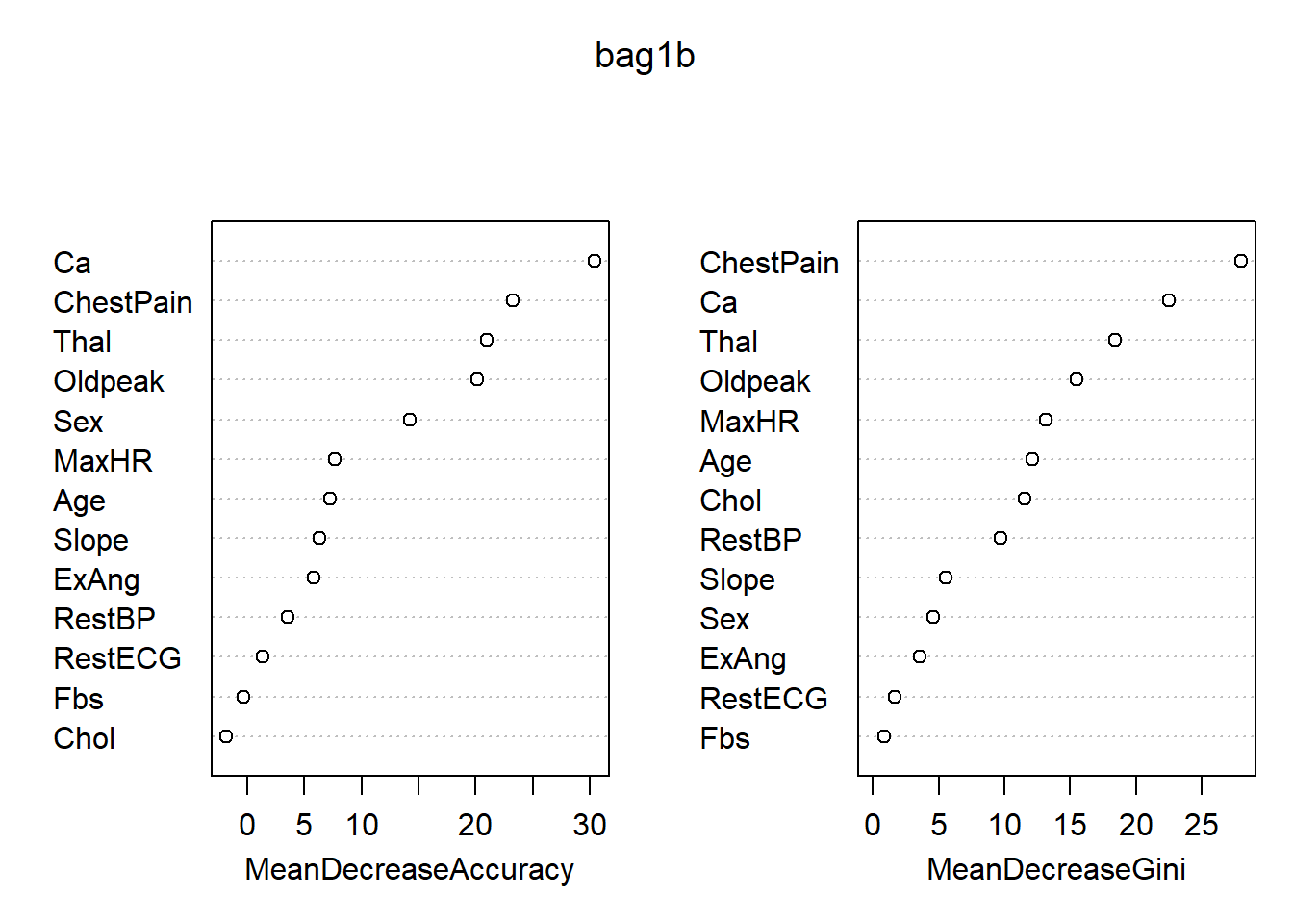

最重要的变量是Thal, ChestPain, Ca。

43.6.4 用随机森林

对训练集用随机森林法：

rf1 <- randomForest(
  AHD ~ ., 
  data = heart_train, 
  importance=TRUE)
rf1

## 
## Call:
##  randomForest(formula = AHD ~ ., data = heart_train, importance = TRUE) 
##                Type of random forest: classification
##                      Number of trees: 500
## No. of variables tried at each split: 3
## 
##         OOB estimate of  error rate: 22.3%
## Confusion matrix:
##     Yes No class.error
## Yes  65 14   0.1772152
## No   19 50   0.2753623

这里mtry取缺省值，对应于随机森林法。

对测试集进行预报:

pred3 <- predict(rf1, newdata = heart_test)
tab3 <- table(pred3, test.y); tab3

##      test.y
## pred3 Yes No
##   Yes  47 15
##   No   11 76

test.err3 <- (tab3[1,2]+tab3[2,1])/sum(tab3[]); test.err3

## [1] 0.1744966

测试集的错判率约为17%。

对全集用随机森林:

rf1b <- randomForest(
  AHD ~ ., 
  data=Heart, 
  importance=TRUE)
rf1b

## 
## Call:
##  randomForest(formula = AHD ~ ., data = Heart, importance = TRUE) 
##                Type of random forest: classification
##                      Number of trees: 500
## No. of variables tried at each split: 3
## 
##         OOB estimate of  error rate: 18.86%
## Confusion matrix:
##     Yes  No class.error
## Yes 108  29   0.2116788
## No   27 133   0.1687500

各变量的重要度数值及其图形：

importance(rf1b)

##                 Yes          No MeanDecreaseAccuracy MeanDecreaseGini
## Age        4.164290  6.96750571           8.73313795        12.987241
## Sex        7.281438 10.61442721          13.05548914         4.987433
## ChestPain 17.452527 11.48126517          19.04415445        18.341807
## RestBP     0.190149  1.37058415           1.24243793        10.526087
## Chol      -2.275121  1.94668809          -0.03619012        11.468039
## Fbs       -1.664923  2.79680029           0.80530655         1.553999
## RestECG    4.645072 -0.02136297           3.19137194         2.815654
## MaxHR      6.711873  8.57257441          10.49071059        17.820488
## ExAng      9.259580  4.60805172           9.61466086         6.847263
## Oldpeak   13.871594  9.53000298          16.91663034        16.497308
## Slope      8.358886  3.06829267           8.36900777         6.832079
## Ca        18.797958 21.81004086          26.74441512        18.984673
## Thal      14.410041 18.71166223          21.30209724        15.882196

varImpPlot(rf1b)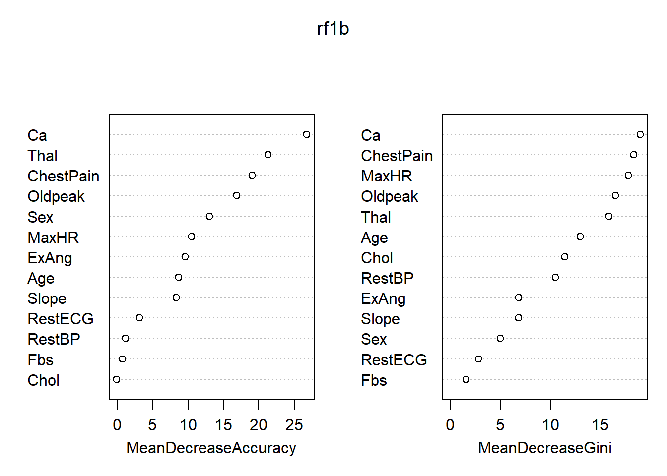

图43.4: Heart数据随机森林方法得到的变量重要度

最重要的变量是Ca, ChestPain。

43.7 附录

43.7.1 Heart数据

knitr::kable(Heart)

Age	Sex	ChestPain	RestBP	Chol	Fbs	RestECG	MaxHR	ExAng	Oldpeak	Slope	Ca	Thal	AHD
63	1	typical	145	233	1	2	150	0	2.3	3	0	fixed	No
67	1	asymptomatic	160	286	0	2	108	1	1.5	2	3	normal	Yes
67	1	asymptomatic	120	229	0	2	129	1	2.6	2	2	reversable	Yes
37	1	nonanginal	130	250	0	0	187	0	3.5	3	0	normal	No
41	0	nontypical	130	204	0	2	172	0	1.4	1	0	normal	No
56	1	nontypical	120	236	0	0	178	0	0.8	1	0	normal	No
62	0	asymptomatic	140	268	0	2	160	0	3.6	3	2	normal	Yes
57	0	asymptomatic	120	354	0	0	163	1	0.6	1	0	normal	No
63	1	asymptomatic	130	254	0	2	147	0	1.4	2	1	reversable	Yes
53	1	asymptomatic	140	203	1	2	155	1	3.1	3	0	reversable	Yes
57	1	asymptomatic	140	192	0	0	148	0	0.4	2	0	fixed	No
56	0	nontypical	140	294	0	2	153	0	1.3	2	0	normal	No
56	1	nonanginal	130	256	1	2	142	1	0.6	2	1	fixed	Yes
44	1	nontypical	120	263	0	0	173	0	0.0	1	0	reversable	No
52	1	nonanginal	172	199	1	0	162	0	0.5	1	0	reversable	No
57	1	nonanginal	150	168	0	0	174	0	1.6	1	0	normal	No
48	1	nontypical	110	229	0	0	168	0	1.0	3	0	reversable	Yes
54	1	asymptomatic	140	239	0	0	160	0	1.2	1	0	normal	No
48	0	nonanginal	130	275	0	0	139	0	0.2	1	0	normal	No
49	1	nontypical	130	266	0	0	171	0	0.6	1	0	normal	No
64	1	typical	110	211	0	2	144	1	1.8	2	0	normal	No
58	0	typical	150	283	1	2	162	0	1.0	1	0	normal	No
58	1	nontypical	120	284	0	2	160	0	1.8	2	0	normal	Yes
58	1	nonanginal	132	224	0	2	173	0	3.2	1	2	reversable	Yes
60	1	asymptomatic	130	206	0	2	132	1	2.4	2	2	reversable	Yes
50	0	nonanginal	120	219	0	0	158	0	1.6	2	0	normal	No
58	0	nonanginal	120	340	0	0	172	0	0.0	1	0	normal	No
66	0	typical	150	226	0	0	114	0	2.6	3	0	normal	No
43	1	asymptomatic	150	247	0	0	171	0	1.5	1	0	normal	No
40	1	asymptomatic	110	167	0	2	114	1	2.0	2	0	reversable	Yes
69	0	typical	140	239	0	0	151	0	1.8	1	2	normal	No
60	1	asymptomatic	117	230	1	0	160	1	1.4	1	2	reversable	Yes
64	1	nonanginal	140	335	0	0	158	0	0.0	1	0	normal	Yes
59	1	asymptomatic	135	234	0	0	161	0	0.5	2	0	reversable	No
44	1	nonanginal	130	233	0	0	179	1	0.4	1	0	normal	No
42	1	asymptomatic	140	226	0	0	178	0	0.0	1	0	normal	No
43	1	asymptomatic	120	177	0	2	120	1	2.5	2	0	reversable	Yes
57	1	asymptomatic	150	276	0	2	112	1	0.6	2	1	fixed	Yes
55	1	asymptomatic	132	353	0	0	132	1	1.2	2	1	reversable	Yes
61	1	nonanginal	150	243	1	0	137	1	1.0	2	0	normal	No
65	0	asymptomatic	150	225	0	2	114	0	1.0	2	3	reversable	Yes
40	1	typical	140	199	0	0	178	1	1.4	1	0	reversable	No
71	0	nontypical	160	302	0	0	162	0	0.4	1	2	normal	No
59	1	nonanginal	150	212	1	0	157	0	1.6	1	0	normal	No
61	0	asymptomatic	130	330	0	2	169	0	0.0	1	0	normal	Yes
58	1	nonanginal	112	230	0	2	165	0	2.5	2	1	reversable	Yes
51	1	nonanginal	110	175	0	0	123	0	0.6	1	0	normal	No
50	1	asymptomatic	150	243	0	2	128	0	2.6	2	0	reversable	Yes
65	0	nonanginal	140	417	1	2	157	0	0.8	1	1	normal	No
53	1	nonanginal	130	197	1	2	152	0	1.2	3	0	normal	No
41	0	nontypical	105	198	0	0	168	0	0.0	1	1	normal	No
65	1	asymptomatic	120	177	0	0	140	0	0.4	1	0	reversable	No
44	1	asymptomatic	112	290	0	2	153	0	0.0	1	1	normal	Yes
44	1	nontypical	130	219	0	2	188	0	0.0	1	0	normal	No
60	1	asymptomatic	130	253	0	0	144	1	1.4	1	1	reversable	Yes
54	1	asymptomatic	124	266	0	2	109	1	2.2	2	1	reversable	Yes
50	1	nonanginal	140	233	0	0	163	0	0.6	2	1	reversable	Yes
41	1	asymptomatic	110	172	0	2	158	0	0.0	1	0	reversable	Yes
54	1	nonanginal	125	273	0	2	152	0	0.5	3	1	normal	No
51	1	typical	125	213	0	2	125	1	1.4	1	1	normal	No
51	0	asymptomatic	130	305	0	0	142	1	1.2	2	0	reversable	Yes
46	0	nonanginal	142	177	0	2	160	1	1.4	3	0	normal	No
58	1	asymptomatic	128	216	0	2	131	1	2.2	2	3	reversable	Yes
54	0	nonanginal	135	304	1	0	170	0	0.0	1	0	normal	No
54	1	asymptomatic	120	188	0	0	113	0	1.4	2	1	reversable	Yes
60	1	asymptomatic	145	282	0	2	142	1	2.8	2	2	reversable	Yes
60	1	nonanginal	140	185	0	2	155	0	3.0	2	0	normal	Yes
54	1	nonanginal	150	232	0	2	165	0	1.6	1	0	reversable	No
59	1	asymptomatic	170	326	0	2	140	1	3.4	3	0	reversable	Yes
46	1	nonanginal	150	231	0	0	147	0	3.6	2	0	normal	Yes
65	0	nonanginal	155	269	0	0	148	0	0.8	1	0	normal	No
67	1	asymptomatic	125	254	1	0	163	0	0.2	2	2	reversable	Yes
62	1	asymptomatic	120	267	0	0	99	1	1.8	2	2	reversable	Yes
65	1	asymptomatic	110	248	0	2	158	0	0.6	1	2	fixed	Yes
44	1	asymptomatic	110	197	0	2	177	0	0.0	1	1	normal	Yes
65	0	nonanginal	160	360	0	2	151	0	0.8	1	0	normal	No
60	1	asymptomatic	125	258	0	2	141	1	2.8	2	1	reversable	Yes
51	0	nonanginal	140	308	0	2	142	0	1.5	1	1	normal	No
48	1	nontypical	130	245	0	2	180	0	0.2	2	0	normal	No
58	1	asymptomatic	150	270	0	2	111	1	0.8	1	0	reversable	Yes
45	1	asymptomatic	104	208	0	2	148	1	3.0	2	0	normal	No
53	0	asymptomatic	130	264	0	2	143	0	0.4	2	0	normal	No
39	1	nonanginal	140	321	0	2	182	0	0.0	1	0	normal	No
68	1	nonanginal	180	274	1	2	150	1	1.6	2	0	reversable	Yes
52	1	nontypical	120	325	0	0	172	0	0.2	1	0	normal	No
44	1	nonanginal	140	235	0	2	180	0	0.0	1	0	normal	No
47	1	nonanginal	138	257	0	2	156	0	0.0	1	0	normal	No
53	0	asymptomatic	138	234	0	2	160	0	0.0	1	0	normal	No
51	0	nonanginal	130	256	0	2	149	0	0.5	1	0	normal	No
66	1	asymptomatic	120	302	0	2	151	0	0.4	2	0	normal	No
62	0	asymptomatic	160	164	0	2	145	0	6.2	3	3	reversable	Yes
62	1	nonanginal	130	231	0	0	146	0	1.8	2	3	reversable	No
44	0	nonanginal	108	141	0	0	175	0	0.6	2	0	normal	No
63	0	nonanginal	135	252	0	2	172	0	0.0	1	0	normal	No
52	1	asymptomatic	128	255	0	0	161	1	0.0	1	1	reversable	Yes
59	1	asymptomatic	110	239	0	2	142	1	1.2	2	1	reversable	Yes
60	0	asymptomatic	150	258	0	2	157	0	2.6	2	2	reversable	Yes
52	1	nontypical	134	201	0	0	158	0	0.8	1	1	normal	No
48	1	asymptomatic	122	222	0	2	186	0	0.0	1	0	normal	No
45	1	asymptomatic	115	260	0	2	185	0	0.0	1	0	normal	No
34	1	typical	118	182	0	2	174	0	0.0	1	0	normal	No
57	0	asymptomatic	128	303	0	2	159	0	0.0	1	1	normal	No
71	0	nonanginal	110	265	1	2	130	0	0.0	1	1	normal	No
49	1	nonanginal	120	188	0	0	139	0	2.0	2	3	reversable	Yes
54	1	nontypical	108	309	0	0	156	0	0.0	1	0	reversable	No
59	1	asymptomatic	140	177	0	0	162	1	0.0	1	1	reversable	Yes
57	1	nonanginal	128	229	0	2	150	0	0.4	2	1	reversable	Yes
61	1	asymptomatic	120	260	0	0	140	1	3.6	2	1	reversable	Yes
39	1	asymptomatic	118	219	0	0	140	0	1.2	2	0	reversable	Yes
61	0	asymptomatic	145	307	0	2	146	1	1.0	2	0	reversable	Yes
56	1	asymptomatic	125	249	1	2	144	1	1.2	2	1	normal	Yes
52	1	typical	118	186	0	2	190	0	0.0	2	0	fixed	No
43	0	asymptomatic	132	341	1	2	136	1	3.0	2	0	reversable	Yes
62	0	nonanginal	130	263	0	0	97	0	1.2	2	1	reversable	Yes
41	1	nontypical	135	203	0	0	132	0	0.0	2	0	fixed	No
58	1	nonanginal	140	211	1	2	165	0	0.0	1	0	normal	No
35	0	asymptomatic	138	183	0	0	182	0	1.4	1	0	normal	No
63	1	asymptomatic	130	330	1	2	132	1	1.8	1	3	reversable	Yes
65	1	asymptomatic	135	254	0	2	127	0	2.8	2	1	reversable	Yes
48	1	asymptomatic	130	256	1	2	150	1	0.0	1	2	reversable	Yes
63	0	asymptomatic	150	407	0	2	154	0	4.0	2	3	reversable	Yes
51	1	nonanginal	100	222	0	0	143	1	1.2	2	0	normal	No
55	1	asymptomatic	140	217	0	0	111	1	5.6	3	0	reversable	Yes
65	1	typical	138	282	1	2	174	0	1.4	2	1	normal	Yes
45	0	nontypical	130	234	0	2	175	0	0.6	2	0	normal	No
56	0	asymptomatic	200	288	1	2	133	1	4.0	3	2	reversable	Yes
54	1	asymptomatic	110	239	0	0	126	1	2.8	2	1	reversable	Yes
44	1	nontypical	120	220	0	0	170	0	0.0	1	0	normal	No
62	0	asymptomatic	124	209	0	0	163	0	0.0	1	0	normal	No
54	1	nonanginal	120	258	0	2	147	0	0.4	2	0	reversable	No
51	1	nonanginal	94	227	0	0	154	1	0.0	1	1	reversable	No
29	1	nontypical	130	204	0	2	202	0	0.0	1	0	normal	No
51	1	asymptomatic	140	261	0	2	186	1	0.0	1	0	normal	No
43	0	nonanginal	122	213	0	0	165	0	0.2	2	0	normal	No
55	0	nontypical	135	250	0	2	161	0	1.4	2	0	normal	No
70	1	asymptomatic	145	174	0	0	125	1	2.6	3	0	reversable	Yes
62	1	nontypical	120	281	0	2	103	0	1.4	2	1	reversable	Yes
35	1	asymptomatic	120	198	0	0	130	1	1.6	2	0	reversable	Yes
51	1	nonanginal	125	245	1	2	166	0	2.4	2	0	normal	No
59	1	nontypical	140	221	0	0	164	1	0.0	1	0	normal	No
59	1	typical	170	288	0	2	159	0	0.2	2	0	reversable	Yes
52	1	nontypical	128	205	1	0	184	0	0.0	1	0	normal	No
64	1	nonanginal	125	309	0	0	131	1	1.8	2	0	reversable	Yes
58	1	nonanginal	105	240	0	2	154	1	0.6	2	0	reversable	No
47	1	nonanginal	108	243	0	0	152	0	0.0	1	0	normal	Yes
57	1	asymptomatic	165	289	1	2	124	0	1.0	2	3	reversable	Yes
41	1	nonanginal	112	250	0	0	179	0	0.0	1	0	normal	No
45	1	nontypical	128	308	0	2	170	0	0.0	1	0	normal	No
60	0	nonanginal	102	318	0	0	160	0	0.0	1	1	normal	No
52	1	typical	152	298	1	0	178	0	1.2	2	0	reversable	No
42	0	asymptomatic	102	265	0	2	122	0	0.6	2	0	normal	No
67	0	nonanginal	115	564	0	2	160	0	1.6	2	0	reversable	No
55	1	asymptomatic	160	289	0	2	145	1	0.8	2	1	reversable	Yes
64	1	asymptomatic	120	246	0	2	96	1	2.2	3	1	normal	Yes
70	1	asymptomatic	130	322	0	2	109	0	2.4	2	3	normal	Yes
51	1	asymptomatic	140	299	0	0	173	1	1.6	1	0	reversable	Yes
58	1	asymptomatic	125	300	0	2	171	0	0.0	1	2	reversable	Yes
60	1	asymptomatic	140	293	0	2	170	0	1.2	2	2	reversable	Yes
68	1	nonanginal	118	277	0	0	151	0	1.0	1	1	reversable	No
46	1	nontypical	101	197	1	0	156	0	0.0	1	0	reversable	No
77	1	asymptomatic	125	304	0	2	162	1	0.0	1	3	normal	Yes
54	0	nonanginal	110	214	0	0	158	0	1.6	2	0	normal	No
58	0	asymptomatic	100	248	0	2	122	0	1.0	2	0	normal	No
48	1	nonanginal	124	255	1	0	175	0	0.0	1	2	normal	No
57	1	asymptomatic	132	207	0	0	168	1	0.0	1	0	reversable	No
54	0	nontypical	132	288	1	2	159	1	0.0	1	1	normal	No
35	1	asymptomatic	126	282	0	2	156	1	0.0	1	0	reversable	Yes
45	0	nontypical	112	160	0	0	138	0	0.0	2	0	normal	No
70	1	nonanginal	160	269	0	0	112	1	2.9	2	1	reversable	Yes
53	1	asymptomatic	142	226	0	2	111	1	0.0	1	0	reversable	No
59	0	asymptomatic	174	249	0	0	143	1	0.0	2	0	normal	Yes
62	0	asymptomatic	140	394	0	2	157	0	1.2	2	0	normal	No
64	1	asymptomatic	145	212	0	2	132	0	2.0	2	2	fixed	Yes
57	1	asymptomatic	152	274	0	0	88	1	1.2	2	1	reversable	Yes
52	1	asymptomatic	108	233	1	0	147	0	0.1	1	3	reversable	No
56	1	asymptomatic	132	184	0	2	105	1	2.1	2	1	fixed	Yes
43	1	nonanginal	130	315	0	0	162	0	1.9	1	1	normal	No
53	1	nonanginal	130	246	1	2	173	0	0.0	1	3	normal	No
48	1	asymptomatic	124	274	0	2	166	0	0.5	2	0	reversable	Yes
56	0	asymptomatic	134	409	0	2	150	1	1.9	2	2	reversable	Yes
42	1	typical	148	244	0	2	178	0	0.8	1	2	normal	No
59	1	typical	178	270	0	2	145	0	4.2	3	0	reversable	No
60	0	asymptomatic	158	305	0	2	161	0	0.0	1	0	normal	Yes
63	0	nontypical	140	195	0	0	179	0	0.0	1	2	normal	No
42	1	nonanginal	120	240	1	0	194	0	0.8	3	0	reversable	No
66	1	nontypical	160	246	0	0	120	1	0.0	2	3	fixed	Yes
54	1	nontypical	192	283	0	2	195	0	0.0	1	1	reversable	Yes
69	1	nonanginal	140	254	0	2	146	0	2.0	2	3	reversable	Yes
50	1	nonanginal	129	196	0	0	163	0	0.0	1	0	normal	No
51	1	asymptomatic	140	298	0	0	122	1	4.2	2	3	reversable	Yes
62	0	asymptomatic	138	294	1	0	106	0	1.9	2	3	normal	Yes
68	0	nonanginal	120	211	0	2	115	0	1.5	2	0	normal	No
67	1	asymptomatic	100	299	0	2	125	1	0.9	2	2	normal	Yes
69	1	typical	160	234	1	2	131	0	0.1	2	1	normal	No
45	0	asymptomatic	138	236	0	2	152	1	0.2	2	0	normal	No
50	0	nontypical	120	244	0	0	162	0	1.1	1	0	normal	No
59	1	typical	160	273	0	2	125	0	0.0	1	0	normal	Yes
50	0	asymptomatic	110	254	0	2	159	0	0.0	1	0	normal	No
64	0	asymptomatic	180	325	0	0	154	1	0.0	1	0	normal	No
57	1	nonanginal	150	126	1	0	173	0	0.2	1	1	reversable	No
64	0	nonanginal	140	313	0	0	133	0	0.2	1	0	reversable	No
43	1	asymptomatic	110	211	0	0	161	0	0.0	1	0	reversable	No
45	1	asymptomatic	142	309	0	2	147	1	0.0	2	3	reversable	Yes
58	1	asymptomatic	128	259	0	2	130	1	3.0	2	2	reversable	Yes
50	1	asymptomatic	144	200	0	2	126	1	0.9	2	0	reversable	Yes
55	1	nontypical	130	262	0	0	155	0	0.0	1	0	normal	No
62	0	asymptomatic	150	244	0	0	154	1	1.4	2	0	normal	Yes
37	0	nonanginal	120	215	0	0	170	0	0.0	1	0	normal	No
38	1	typical	120	231	0	0	182	1	3.8	2	0	reversable	Yes
41	1	nonanginal	130	214	0	2	168	0	2.0	2	0	normal	No
66	0	asymptomatic	178	228	1	0	165	1	1.0	2	2	reversable	Yes
52	1	asymptomatic	112	230	0	0	160	0	0.0	1	1	normal	Yes
56	1	typical	120	193	0	2	162	0	1.9	2	0	reversable	No
46	0	nontypical	105	204	0	0	172	0	0.0	1	0	normal	No
46	0	asymptomatic	138	243	0	2	152	1	0.0	2	0	normal	No
64	0	asymptomatic	130	303	0	0	122	0	2.0	2	2	normal	No
59	1	asymptomatic	138	271	0	2	182	0	0.0	1	0	normal	No
41	0	nonanginal	112	268	0	2	172	1	0.0	1	0	normal	No
54	0	nonanginal	108	267	0	2	167	0	0.0	1	0	normal	No
39	0	nonanginal	94	199	0	0	179	0	0.0	1	0	normal	No
53	1	asymptomatic	123	282	0	0	95	1	2.0	2	2	reversable	Yes
63	0	asymptomatic	108	269	0	0	169	1	1.8	2	2	normal	Yes
34	0	nontypical	118	210	0	0	192	0	0.7	1	0	normal	No
47	1	asymptomatic	112	204	0	0	143	0	0.1	1	0	normal	No
67	0	nonanginal	152	277	0	0	172	0	0.0	1	1	normal	No
54	1	asymptomatic	110	206	0	2	108	1	0.0	2	1	normal	Yes
66	1	asymptomatic	112	212	0	2	132	1	0.1	1	1	normal	Yes
52	0	nonanginal	136	196	0	2	169	0	0.1	2	0	normal	No
55	0	asymptomatic	180	327	0	1	117	1	3.4	2	0	normal	Yes
49	1	nonanginal	118	149	0	2	126	0	0.8	1	3	normal	Yes
74	0	nontypical	120	269	0	2	121	1	0.2	1	1	normal	No
54	0	nonanginal	160	201	0	0	163	0	0.0	1	1	normal	No
54	1	asymptomatic	122	286	0	2	116	1	3.2	2	2	normal	Yes
56	1	asymptomatic	130	283	1	2	103	1	1.6	3	0	reversable	Yes
46	1	asymptomatic	120	249	0	2	144	0	0.8	1	0	reversable	Yes
49	0	nontypical	134	271	0	0	162	0	0.0	2	0	normal	No
42	1	nontypical	120	295	0	0	162	0	0.0	1	0	normal	No
41	1	nontypical	110	235	0	0	153	0	0.0	1	0	normal	No
41	0	nontypical	126	306	0	0	163	0	0.0	1	0	normal	No
49	0	asymptomatic	130	269	0	0	163	0	0.0	1	0	normal	No
61	1	typical	134	234	0	0	145	0	2.6	2	2	normal	Yes
60	0	nonanginal	120	178	1	0	96	0	0.0	1	0	normal	No
67	1	asymptomatic	120	237	0	0	71	0	1.0	2	0	normal	Yes
58	1	asymptomatic	100	234	0	0	156	0	0.1	1	1	reversable	Yes
47	1	asymptomatic	110	275	0	2	118	1	1.0	2	1	normal	Yes
52	1	asymptomatic	125	212	0	0	168	0	1.0	1	2	reversable	Yes
62	1	nontypical	128	208	1	2	140	0	0.0	1	0	normal	No
57	1	asymptomatic	110	201	0	0	126	1	1.5	2	0	fixed	No
58	1	asymptomatic	146	218	0	0	105	0	2.0	2	1	reversable	Yes
64	1	asymptomatic	128	263	0	0	105	1	0.2	2	1	reversable	No
51	0	nonanginal	120	295	0	2	157	0	0.6	1	0	normal	No
43	1	asymptomatic	115	303	0	0	181	0	1.2	2	0	normal	No
42	0	nonanginal	120	209	0	0	173	0	0.0	2	0	normal	No
67	0	asymptomatic	106	223	0	0	142	0	0.3	1	2	normal	No
76	0	nonanginal	140	197	0	1	116	0	1.1	2	0	normal	No
70	1	nontypical	156	245	0	2	143	0	0.0	1	0	normal	No
57	1	nontypical	124	261	0	0	141	0	0.3	1	0	reversable	Yes
44	0	nonanginal	118	242	0	0	149	0	0.3	2	1	normal	No
58	0	nontypical	136	319	1	2	152	0	0.0	1	2	normal	Yes
60	0	typical	150	240	0	0	171	0	0.9	1	0	normal	No
44	1	nonanginal	120	226	0	0	169	0	0.0	1	0	normal	No
61	1	asymptomatic	138	166	0	2	125	1	3.6	2	1	normal	Yes
42	1	asymptomatic	136	315	0	0	125	1	1.8	2	0	fixed	Yes
59	1	nonanginal	126	218	1	0	134	0	2.2	2	1	fixed	Yes
40	1	asymptomatic	152	223	0	0	181	0	0.0	1	0	reversable	Yes
42	1	nonanginal	130	180	0	0	150	0	0.0	1	0	normal	No
61	1	asymptomatic	140	207	0	2	138	1	1.9	1	1	reversable	Yes
66	1	asymptomatic	160	228	0	2	138	0	2.3	1	0	fixed	No
46	1	asymptomatic	140	311	0	0	120	1	1.8	2	2	reversable	Yes
71	0	asymptomatic	112	149	0	0	125	0	1.6	2	0	normal	No
59	1	typical	134	204	0	0	162	0	0.8	1	2	normal	Yes
64	1	typical	170	227	0	2	155	0	0.6	2	0	reversable	No
66	0	nonanginal	146	278	0	2	152	0	0.0	2	1	normal	No
39	0	nonanginal	138	220	0	0	152	0	0.0	2	0	normal	No
57	1	nontypical	154	232	0	2	164	0	0.0	1	1	normal	Yes
58	0	asymptomatic	130	197	0	0	131	0	0.6	2	0	normal	No
57	1	asymptomatic	110	335	0	0	143	1	3.0	2	1	reversable	Yes
47	1	nonanginal	130	253	0	0	179	0	0.0	1	0	normal	No
55	0	asymptomatic	128	205	0	1	130	1	2.0	2	1	reversable	Yes
35	1	nontypical	122	192	0	0	174	0	0.0	1	0	normal	No
61	1	asymptomatic	148	203	0	0	161	0	0.0	1	1	reversable	Yes
58	1	asymptomatic	114	318	0	1	140	0	4.4	3	3	fixed	Yes
58	0	asymptomatic	170	225	1	2	146	1	2.8	2	2	fixed	Yes
56	1	nontypical	130	221	0	2	163	0	0.0	1	0	reversable	No
56	1	nontypical	120	240	0	0	169	0	0.0	3	0	normal	No
67	1	nonanginal	152	212	0	2	150	0	0.8	2	0	reversable	Yes
55	0	nontypical	132	342	0	0	166	0	1.2	1	0	normal	No
44	1	asymptomatic	120	169	0	0	144	1	2.8	3	0	fixed	Yes
63	1	asymptomatic	140	187	0	2	144	1	4.0	1	2	reversable	Yes
63	0	asymptomatic	124	197	0	0	136	1	0.0	2	0	normal	Yes
41	1	nontypical	120	157	0	0	182	0	0.0	1	0	normal	No
59	1	asymptomatic	164	176	1	2	90	0	1.0	2	2	fixed	Yes
57	0	asymptomatic	140	241	0	0	123	1	0.2	2	0	reversable	Yes
45	1	typical	110	264	0	0	132	0	1.2	2	0	reversable	Yes
68	1	asymptomatic	144	193	1	0	141	0	3.4	2	2	reversable	Yes
57	1	asymptomatic	130	131	0	0	115	1	1.2	2	1	reversable	Yes
57	0	nontypical	130	236	0	2	174	0	0.0

北京大学R语言教程(李东风)第43章：基于树的方法

43.1 树回归的简单演示

43.2 树回归

43.3 装袋法

43.4 随机森林

43.5 提升法

43.6 心脏病诊断建模预报

43.6.1 划分训练集与测试集

43.6.2 判别树

43.6.2.1 适当剪枝

43.6.2.2 对测试集计算误判率

43.6.2.3 利用全集数据建立剪枝判别树

43.6.3 用装袋法

43.6.4 用随机森林

43.7 附录

43.7.1 Heart数据

相关推荐

北京大学R语言教程(李东风)第40章： 随机模拟

日本股市的春天

为什么必须优先考虑最大限度地降低投资产品的成本？

长期、低息国债很有吸引力

北京大学金融时间序列分析讲义第20章： 随机波动率模型

发表回复

北京大学R语言教程(李东风)第40章：随机模拟

北京大学金融时间序列分析讲义第20章：随机波动率模型